Polarization and Entanglement 偏振和纠缠
Abstract 摘要
As our understanding of the physical world grew so did our theories to keep with new findings and observations. In many cases this transition is not always smooth. One such case is the growing field of quantum mechanics whose strange postulates puzzled physicists for decades. Until recently, it was often debated whether quantum mechanics was really necessary - or whether everything can be explained through classical mechanics alone. In additional to laying the groundwork in understanding the nature of entangled photon states we will also provide experimental evidence using spontaneous parametric down-conversion to both refute local hidden variable theories and support the existing quantum mechanical framework.
随着我们对物理世界认识的加深,我们的理论也在不断发展以适应新的发现和观察。在许多情况下,这种转变并不总是平稳的。其中一个例子就是正在发展的量子力学领域,其奇特的假设困扰了物理学家数十年。直到最近,人们仍在争论量子力学是否真的必要 - 或者是否一切都可以仅通过经典力学来解释。除了为理解纠缠光子态的本质奠定基础外,我们还将使用自发参量下转换提供实验证据,以驳斥局域隐变量理论并支持现有的量子力学框架。
随着我们对物理世界的理解不断深入,我们的理论体系也在不断演化,以便能够更好地解释和预测新的实验结果和观察现象。然而,这种理论演进的过程并不总是一帆风顺的。在科学发展的历史中,许多新的理论往往是对旧有理论的一种补充、扩展甚至是颠覆,而这类变革通常会引发长时间的争论和探索。
其中,量子力学的兴起便是一个典型的例子。量子力学的发展是20世纪物理学最重要的变革之一,其基本假设和数学框架在很大程度上颠覆了经典物理学的直觉。量子力学提出了一系列极为反常的概念,例如波粒二象性、不确定性原理、量子叠加态和量子纠缠等,这些概念与我们在日常生活中的经验和经典力学的描述大相径庭。因此,自量子力学诞生以来,它便成为科学界激烈争论的焦点,物理学家们试图理解其深层含义,并探讨它是否确实是对自然界更准确的描述。
事实上,在相当长的一段时间里,许多科学家并不完全接受量子力学,甚至有人试图寻找可能的替代理论。例如,一些物理学家认为,量子力学或许只是对世界的一种近似描述,而真正的物理规律应该仍然遵循经典力学的因果性和确定性原则。这种观点催生了一类被称为局域隐变量理论(local hidden variable theories)的尝试。这些理论认为,量子力学中的概率性和不确定性只是表象,而实际上,存在一些尚未探测到的“隐变量”,它们在幕后决定了微观粒子的真实状态。如果这些隐变量能够被发现并加以测量,那么我们或许仍然可以用经典方式来描述量子现象,从而避免量子力学中的种种反直觉特性。
然而,随着科学实验技术的发展,物理学家逐渐获得了越来越多的实验证据,这些证据表明量子力学并非仅仅是一种数学上的巧合,而是对物理世界本质更加准确的刻画。其中,最引人注目的实验之一是基于自发参量下转换(Spontaneous Parametric Down-Conversion, SPDC)现象的实验。自发参量下转换是一种非线性光学过程,其中一个高能光子在某些特殊的非线性介质(如某些晶体)中会自发地分裂成两个能量较低、但具有特定相干性和纠缠特性的光子。这些纠缠光子对的产生,使得物理学家能够设计精确的实验,来测试量子力学的预言是否成立,以及是否存在隐变量理论能够替代量子力学的描述。
通过这些实验,科学家们不仅成功展示了量子纠缠的真实性,还直接证伪了许多局域隐变量理论的预测。这些实验表明,量子力学所描述的非定域(non-local)现象是客观存在的,粒子之间的关联性无法通过经典信息传播的方式来解释。这些研究为量子力学的理论基础提供了强有力的支持,也促使科学界逐步接受量子力学作为描述微观世界的最基本框架。
综上所述,量子力学的提出和发展并非一蹴而就,而是伴随着长期的探索、争议和实验检验。在本研究中,我们不仅致力于为理解纠缠光子态的本质奠定理论基础,还通过自发参量下转换实验提供直接证据,以此进一步驳斥局域隐变量理论,并巩固现有的 量子力学框架 。这一系列研究对于深入理解量子世界的本质,以及未来在量子通信、量子计算等领域的发展,均具有重要的科学价值和实际应用意义。
I. Introduction I. 引言
Since its birth in the early 1900s till the later half of the century, quantum mechanics was never accepted as a rigorous and meaningful theory. Unlike the results of classical mechanics and electrodynamics, quantum mechanics seemed as an almost strange and unnatural theory. How could basic information such as position and momentum of a particle not be known until it is measured? How can entangled states transmit information faster than light speed? How can a cat in a box be both dead and alive? While we are now more comfortable with these questions as the field of quantum mechanics has matured, these same unintuitive questions puzzled and even repulsed many prominent physicists of the last century.
自20世纪初诞生直到本世纪后半叶,量子力学一直未被接受为一个严格和有意义的理论。与经典力学和电动力学的结果不同,量子力学似乎是一个几乎陌生和不自然的理论。为什么粒子的基本信息如位置和动量在测量之前是未知的?为什么纠缠态能以超光速传递信息?为什么盒子里的猫可以同时是死的和活的?虽然随着量子力学领域的成熟,我们现在对这些问题更加适应,但这些反直觉的问题曾经困扰甚至排斥了上个世纪的许多杰出物理学家。
The biggest hurdle to any theory is that is can never be accepted until it has been rigorously and thoroughly tested through experiments. For quantum mechanics this is no different. Over the course of this paper, we will provide groundwork for understanding the complex nature of polarization and how entangled photons pairs can be produced using spontaneous parametric down conversion (SPDC). We will explore how density matrices of multiqubit systems can be reconstructed using quantum state tomography and culminate with experimental evidence supporting the theory of quantum with Bell's Inequality.
任何理论最大的障碍在于,在经过严格和全面的实验检验之前,它永远不会被接受。对于量子力学来说也不例外。在本文中,我们将为理解偏振的复杂本质以及如何使用自发参量下转换(SPDC)产生纠缠光子对奠定基础。我们将探讨如何使用量子态层析重建多量子比特系统的密度矩阵,并以支持量子理论的实验证据和贝尔不等式作为culmination。
The remainder of the paper will be structured as follows. Section II will provide an overview of the polarization of light and how it transforms in optical elements through Jones calculus. Section III will discuss the generation and entanglement quality of entangled photon pairs via SPDC. Sections IV and V will explore how coincidence measurements can be used to reconstruct density matrices and reinforce the packet-like nature of photons respectively. Section VI will investigate Bell's inequality and provide experimental evidence for quantum mechanics. Section VII will conclude.
本文的其余部分结构如下。第二节将概述光的偏振及其通过琼斯算法在光学元件中的转换。第三节将讨论通过SPDC产生的纠缠光子对的产生和纠缠质量。第四和五节将分别探讨如何使用符合测量来重建密度矩阵并加强光子的包状本质。第六节将研究贝尔不等式并为量子力学提供实验证据。第七节将总结全文。
自 20 世纪初 量子力学 诞生以来,直到本世纪的后半叶,它一直未能被广泛接受为一个严格且具有现实意义的理论体系。相比于 经典力学 和 电动力学 所提供的直观且符合人类日常经验的结果,量子力学 似乎更像是一种奇异且反直觉的数学描述。这种不自然性使得许多物理学家在面对 量子力学 的基本原理时感到困惑,甚至对其提出质疑。
在 经典物理学 中,物体的运动状态由其 位置、速度 和 加速度 等物理量完全确定,并且这些量可以通过测量获得明确的数值。然而,在 量子力学 框架下,基本粒子如 电子 或 光子 并不像经典粒子那样具有确定的 位置 和 动量。根据 海森堡不确定性原理,粒子的 位置 和 动量 无法同时被精确测定。这一理论挑战了 经典物理学 关于物理世界确定性的基本假设。物理学家不禁要问:“为什么粒子的基本信息,如 位置 和 动量,在测量之前是未知的?它们是否真的‘存在’,还是测量本身在某种意义上‘创造’了这些属性?”
另一个令物理学家困惑的问题是 量子纠缠 现象。根据 量子力学 的描述,当两个或多个粒子处于一种特殊的 量子态(即 纠缠态)时,其中一个粒子的状态测量结果会立即影响另一个粒子的状态,即使它们相隔极远。爱因斯坦等物理学家提出:“如果 量子力学 是正确的,那么它意味着存在某种‘超光速’的信息传递方式。” 这与 相对论 的基本原理直接冲突,因此爱因斯坦、波多尔斯基和罗森在 1935 年提出了著名的 EPR 佯谬,试图说明 量子力学 的描述是不完备的,可能存在某种隐藏的变量(即所谓的 隐变量理论),使得 量子力学 看似随机的结果其实可以用 经典方式 进行解释。然而,后来的研究和实验表明,量子纠缠 现象并非 隐变量理论 所能描述,而是 量子力学 固有的特性。
更极端的例子是著名的 薛定谔的猫 思想实验。薛定谔在这一实验中构造了一个极端的情境——一个密闭的盒子中放置了一只猫,同时盒子里还包含一个 放射性原子 和一个 检测装置。如果该 原子 发生衰变,它会触发一个机制杀死猫,否则猫会存活。根据 量子力学 的解释,在未打开盒子之前,猫的状态应该是 衰变 与 未衰变 的叠加态,也就是说,猫应该是“死的”和“活的”同时存在的。然而,在我们的日常经验中,物体只能处于某个确定的状态,而不可能同时处于多个状态。这一悖论式的问题曾让许多物理学家感到不适,甚至拒绝接受 量子力学 的描述。
然而,尽管 量子力学 看似反直觉,科学的黄金法则是:任何理论的最终检验标准是实验,而不是直觉。一个理论是否被接受,关键在于它是否能够经受住严格和全面的 实验检验,而非其是否符合人类的直觉认知。对于 量子力学 来说也是如此。随着 20 世纪后半叶一系列高精度实验的开展,量子力学 的诸多奇异预言得到了实验证实,使得它逐渐从一种令人困惑的数学模型,发展成为描述自然界的基本理论之一。
在本文中,我们将系统地探讨 量子力学 的一些关键概念,并通过实验验证其理论预测。
1 首先,我们将介绍 偏振 这一重要的物理现象,并讨论 光 在不同 光学元件 中的传播如何通过 琼斯矩阵(Jones Calculus) 进行描述。
2 接着,我们会介绍如何利用 自发参量下转换(SPDC, Spontaneous Parametric Down-Conversion) 这一 非线性光学 过程来产生一对 纠缠光子,并分析这些 光子 的 纠缠质量。
3 在理解了 光子 的 偏振 和 纠缠态 后,我们将探讨如何使用 量子态层析技术(Quantum State Tomography) 来重建 多量子比特系统的密度矩阵,从而获得对 量子态 更精确的描述。
4 随后,我们会讨论 符合测量(Coincidence Measurement) 在 量子力学实验 中的应用,并分析这些实验如何进一步证明 光子 的 波粒二象性 以及其“包状”特性,即 光子 既可以表现出 波动性,又可以表现出 粒子性。
5 最后,我们将在本文的结尾部分详细研究 贝尔不等式(Bell's Inequality),并通过 实验数据 来检验 量子力学 的正确性。贝尔不等式 是检验 局域隐变量理论 与 量子力学 之间矛盾的关键数学工具。根据 贝尔定理,如果自然界确实是由 隐变量 决定的,那么 实验数据 应该符合 贝尔不等式 的预测;而如果 量子力学 的 非定域性 描述是正确的,那么 实验数据 将会违反 贝尔不等式。现代物理实验已经反复证明,贝尔不等式 确实被违反,这为 量子力学 的正确性提供了最直接的 实验支持,并且进一步证伪了 局域隐变量理论。
本文的结构安排如下:
1 第二节 将介绍 光的偏振特性,以及如何利用 琼斯矩阵 描述 偏振光 在不同 光学元件 中的演化。
2 第三节 讨论 纠缠光子 的产生方法,重点介绍 自发参量下转换(SPDC) 技术及其在实验中的应用。
3 第四节 介绍如何使用 符合测量 来重建 多量子比特系统的密度矩阵,并分析 密度矩阵 在 量子信息处理 中所扮演的角色。
4 第五节 进一步探讨 光子 的 量子特性,并通过 实验数据 验证 光子 的 波粒二象性。
5 第六节 研究 贝尔不等式,并展示通过 实验数据 如何检验 量子力学 的正确性。
第七节 对全文进行总结,并讨论未来研究的方向。
综上所述,量子力学从最初的不被接受,到如今成为现代物理学的支柱理论,经历了漫长的实验验证和科学探索。尽管其基本概念仍然反直觉,但实验已经证明了量子力学的正确性和必要性。通过本文的研究,我们不仅希望加深对量子态和纠缠态的理解,也希望通过实验证据巩固量子力学的理论框架,为未来的量子计算、量子通信等领域的发展奠定基础。
II. Polarization II. 偏振
Before exploring the quantum mechanical nature of light, it is important to first establish an understanding of the electro-magnetic fields of light, formalized by Maxwell in the late 19th century, and its evolution under various optical apparatuses. Suppose we have a linearly polarized beam of light propagating in the direction. Its electric field can be written as
在探索光的量子力学本质之前,首先建立对光的电磁场的理解是很重要的,这是由麦克斯韦在19世纪末正式提出的,以及它在各种光学仪器下的演化。假设我们有一束在方向传播的线性偏振光。其电场可以写作
if it's polarized along the x axis or
如果它沿x轴偏振,或
if it's polarized along the y axis where is some proportionality constant, k is the wavenumber and is the angular frequency.
如果它沿y轴偏振,其中是某个比例常数,k是波数,是角频率。
在探索光的 量子力学 本质之前,首先建立对光的 电磁场 的理解是至关重要的。光的 电磁场 由 麦克斯韦(Maxwell) 在 19 世纪末正式提出并通过 麦克斯韦方程组 进行数学描述。电磁波 的传播不仅受到 经典电动力学 规律的支配,同时在光学实验中,光的 偏振特性 也扮演着至关重要的角色。在理解 偏振光 的行为之前,我们需要先了解光的 电场分量 如何随时间和空间变化,并分析其在各种 光学元件 中的演化。
线性偏振光的电场E描述
假设我们有一束沿 方向传播的线性偏振光。线性偏振光是指光的电场矢量在传播方向上始终沿固定方向振荡,而磁场矢量则与之垂直。
如果光的偏振方向沿 x 轴,则其电场可以用以下数学表达式表示:
其中:
- :表示电场振幅,即最大电场强度。
- :表示波数,定义为 ,其中 是光的波长。
- :表示角频率,定义为 ,其中 是光的频率。
- :描述电场随时间和空间的传播行为。
- :单位矢量,表示电场振荡的方向。
如果光的偏振方向沿 y 轴,则其电场可以用类似的数学表达式表示:
在这种情况下:
- 电场矢量沿 y 轴方向振荡,而磁场矢量垂直于电场和传播方向(即沿 x 轴)。
- 其他变量(, , )的物理意义与 x 轴偏振相同。
偏振光的基本特性
- 线性偏振光:光的电场矢量始终沿某一固定方向振荡,不随时间改变。
- 圆偏振光:电场矢量的方向在传播过程中以恒定角速度旋转,形成顺时针或逆时针的螺旋形轨迹。
- 椭圆偏振光:电场矢量的端点轨迹呈现椭圆形,是线性偏振光与圆偏振光的推广形式。
在实际光学实验中,利用 偏振片、波片(如四分之一波片和二分之一波片) 以及 棱镜 可以有效地操控光的偏振态,从而实现对光学系统的精确控制。
A. Jones Calculus A. 琼斯算法
In general, linearly polarized light does not strictly have to be polarized along the x or y directions and instead can take any normalized combination of the two. Let us characterize the polarization using a compact unit vector that lives on the xy plane such that we can write
一般来说,线性偏振光并不严格要求沿x或y方向偏振,而是可以取这两个方向的任意归一化组合。让我们用一个生活在xy平面上的紧凑单位矢量来表征这种偏振,使得我们可以写作
for linearly polarized light along some arbitrary axis . More precisely, let us orient our xy plane such that anything polarized along has horizontal polarization and anything polarized along has vertical polarization such that
对于沿任意轴的线性偏振光。更准确地说,让我们定向我们的xy平面,使得沿偏振的任何东西具有水平偏振,沿偏振的任何东西具有垂直偏振,使得
where is proportional to the amplitude of the electric field that is horizontally (vertically) polarized subject to the normalization condition that . For instance, a pure horizontally polarized beam would have is commonly known as a Jones vector and we will in the coming sections that its components may be complex.
其中与水平(垂直)偏振的电场振幅成正比,服从归一化条件 。例如,一个纯水平偏振的光束会有。通常被称为琼斯矢量,我们将在接下来的章节中看到它的分量可能是复数。
B. Jones Matrices B. 琼斯矩阵
In addition to being a compact way of representing arbitrary polarization on the xy plane, Jones vectors also evolve nicely as the beam propagates through various polarizers and optical elements. More precisely, an optical element can be characterized by its Jones matrix and transforms Jones vectors in the standard way: . Since Jones matrices are determined entirely by the properties of the optical element and does not depend on the properties of light, they can be formalized as a linear system such that the Jones vector transforms through multiple optical elements with matrices in the natural way:
除了是表示xy平面上任意偏振的紧凑方式外,当光束通过各种偏振器和光学元件传播时,琼斯矢量也能很好地演化。更准确地说,一个光学元件可以用其的琼斯矩阵来表征,并以标准方式变换琼斯矢量:。由于琼斯矩阵完全由光学元件的性质决定,而不依赖于光的性质,它们可以被形式化为一个线性系统,使得琼斯矢量通过多个具有矩阵的光学元件以自然方式变换:
Given a Jones matrix T for some optical element, it is also simple to compute its transformed matrix after the optical element has been rotated by some angle . More precisely, for a rotation in the axis by angle , the transformed matrix is given by
对于某个光学元件的琼斯矩阵T,在光学元件旋转某个角度后计算其变换矩阵也很简单。更准确地说,对于沿轴旋转角度,变换矩阵由下式给出
where
is the standard 2 x 2 rotation matrix.
是标准的2 x 2旋转矩阵。
C. Polarizers and Wave Plates C. 偏振器和波片
The optical elements that are used in this lab consists of 5050 beamsplitters (equivalently a horizontal and vertical polarizer), linear polarizers, half wave plates (HWP) and quarter wave plates (QWP). As their name suggests, linear polarizers only allow light polarized along the direction of polarization to pass. For example, a horizontal polarizer has Jones matrix
本实验中使用的光学元件包括5050分束器(相当于一个水平和垂直偏振器)、线性偏振器、半波片(HWP)和四分之一波片(QWP)。顾名思义,线性偏振器只允许沿偏振方向偏振的光通过。例如,水平偏振器的琼斯矩阵为
For a linear polarizer along an angle from the horizontal, its Jones matrix is
对于从水平方向旋转角度的线性偏振器,其琼斯矩阵为
Indeed, for reduces to the Jones matrix of a vertical polarizer:
实际上,当时,9式简化为垂直偏振器的琼斯矩阵:
For HWPs and QWPs, these optical elements operate by changing the wavelengths and wave-numbers of light along its fast and slow axes. More precisely, light polarized along the fast axis have longer wavelength and smaller wavenumber than light polarized along the slow axis. This effectively generates a phase difference between the horizontal and vertical polarization amplitudes and which can be used to generate arbitrary linearly polarized light with HWPs and elliptically polarized light with QEPs. When used together, they can be used to generate arbitrary polarizations. The Jones matrices for HWPs and QWPs with their fast axis aligned along the vertical are
对于HWP和QWP,这些光学元件通过改变沿其快轴和慢轴的光的波长和波数来工作。更准确地说,沿快轴偏振的光具有比沿慢轴偏振的光更长的波长和更小的波数。这有效地在水平和垂直偏振幅度 和 之间产生相位差,可用于用HWP产生任意的线性偏振光,用QEP产生椭圆偏振光。当它们一起使用时,可以产生任意的偏振。当快轴沿垂直方向对齐时,HWP和QWP的琼斯矩阵分别为
for HWPs and
对于HWP:
for QWPs. For HWPs and QWPs rotated in the direction by angle , their generalized Jones matrices can be shown to be
对于QWP。对于在方向旋转角度的HWP和QWP,它们的广义琼斯矩阵可以表示为
and
和
respectively.
分别。
D. Crossed Polarizers****交叉偏振器
To experimentally explore polarization and the Jones calculus formalism, we analyzed how unpolarized laser light transformed as it propagated through various setups of polarizers, waveplates and beamsplitters. The laser and linear polarizers used in this experiment had an extinction ratio of as the polarizer was rotated in the unpolarized beam path. The transmissions when a pair of linear polarizers are aligned and anti-aligned are 10.504 V and 282 mV respectively. While the polarizers and laser light used in this lab weren't of the highest quality, they will suffice for the purpose of exploring and understanding the evolution of polarization. To this end, consider the setup of two orthogonally aligned linear polarizers with a central polarizer that is free to rotate. When the central polarizer is rotated an angle from the horizontal, the Jones matrix describing the system is
为了实验探索偏振和琼斯算法形式,我们分析了未偏振的激光在通过各种偏振器、波片和分束器装置时如何转变。本实验中使用的激光器和线性偏振器在偏振器在未偏振光束路径中旋转时具有的消光比。当一对线性偏振器对齐和反对齐时,透射率分别为10.504 V和282 mV。虽然本实验中使用的偏振器和激光质量不是最高的,但足以用于探索和理解偏振的演化。为此,考虑两个正交对齐的线性偏振器的装置,其中有一个可自由旋转的中心偏振器。当中心偏振器从水平方向旋转角度时,描述该系统的琼斯矩阵为
For an incoming beam with Jones vector , the Jones vector after the system is
对于入射的光束,其琼斯矢量为,该系统输出的琼斯矢量为
Measuring the transmitted intensity with a photodetector at the end of the system, we expect that the intensity evolves as where intensity is proportional to the absolute value squared of the electric field. Indeed, the experimental data agrees well with theory with transmitted power .
使用光电探测器在系统末端测量透射光强,我们预期光强随演化,其中光强与电场的绝对值平方成正比。实际上,实验数据与理论预测的透射功率符合得很好。
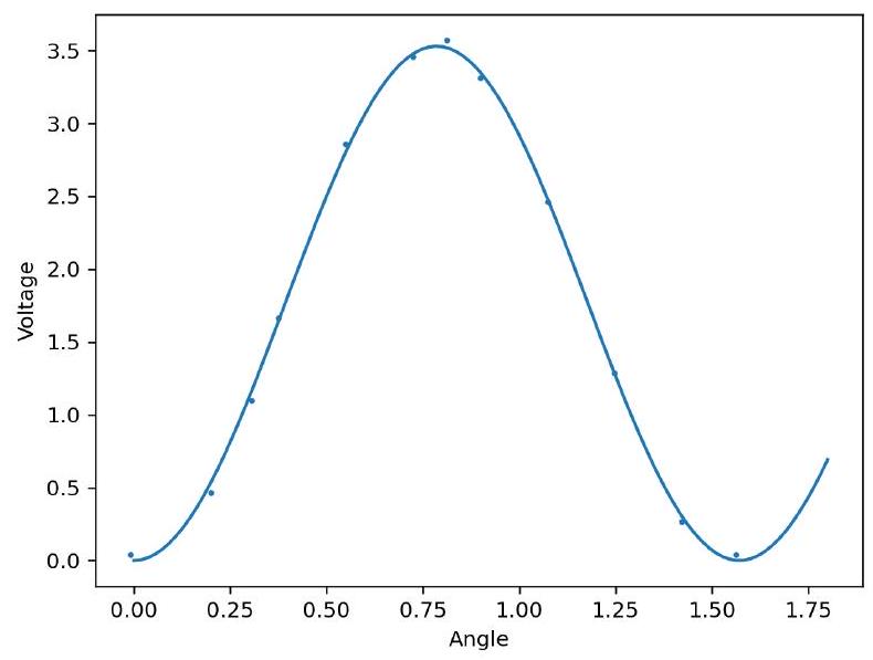
FIG. 1. Transmitted intensity of orthogonal linear polarizers with a central rotating polarizer as a function of the central polarizer angle. The experimental data (points) are fit to the equation for angle x.
图1. 正交线性偏振器中心旋转偏振器的透射光强随中心偏振器角度的变化关系。实验数据点拟合方程为,其中x为角度。
E. Waveplates E. 波片
To explore the behavior of waveplates, consider the system of a waveplate sandwiched between two polarizing beamsplitters (PBS) with photodetectors at both outputs of the final beamsplitter. The initial PBS polarizes the laser light in a known linear polarization before it enters the waveplate. The final PBS splits the polarized light into horizontal and vertical components that we can then measure with photodetectors.
为了探究波片的行为,考虑一个由两个偏振分束器(PBS)夹住波片的系统,在最后一个分束器的两个输出端各放置一个光电探测器。初始PBS在光进入波片之前将激光偏振成已知的线性偏振。最后的PBS将偏振光分成水平和垂直分量,然后我们可以用光电探测器测量。
For a HWP with its fast axis rotated by angle from the vertical, its Jones matrix is ?? as discussed above. For incoming horizontally polarized light, the transformed Jones vector is
对于快轴从垂直方向旋转角度的半波片(HWP),其琼斯矩阵如上所述为??。对于入射的水平偏振光,变换后的琼斯矢量为
After the beam is split by the final beamspliter, we expect to measure transmitted powers of and at each photodetector. From figure 2, we see that the experimental results agree well with theory.
在光束被最后的分束器分开后,我们预期在每个光电探测器处测量到的透射功率分别为和。从图2可以看出,实验结果与理论符合得很好。
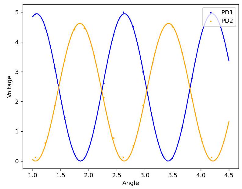
FIG. 2. Transmitted intensities of a rotated HWP at each output of a polarizing beam splitter. The experimental data for PD1 (blue) is fit to and for PD2. Fast axis at 60 degrees 1.047 rad.
图2. 旋转半波片在偏振分束器每个输出端的透射光强。光电探测器1(PD1)(蓝色)的实验数据拟合为,光电探测器2(PD2)拟合为。快轴在60度 1.047弧度。
For a QWP with its fast axis rotated by angle from the vertical, a similar calculation shows that an incoming horizontally polarized beam transforms as
对于快轴从垂直方向旋转角度的四分之一波片(QWP),类似的计算表明入射的水平偏振光束变换为
such that the transmitted powers at the photodetectors are and . Indeed from figure 3, we see that this agrees with experimental results.
因此在光电探测器处测量到的透射功率为 和 。从图3可以看出,这与实验结果符合。
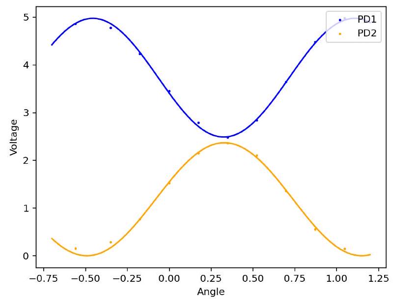
FIG. 3. Transmitted intensities of a rotated QWP at each output of a polarizing beam splitter. The experimental data for PD1 (blue) is fit to and for PD2. Fast axis at 328 degrees
图3. 旋转四分之一波片在偏振分束器每个输出端的透射光强。光电探测器1(PD1)(蓝色)的实验数据拟合为 ,光电探测器2(PD2)拟合为。快轴在328度弧度。
From the figure above, we notice that that the intensities nearly match at certain angles of the QWP. More specifically, for a QWP with fast axis rotated by angle from the vertical, it transforms horizontally polarized light into what is known as circularly polarized light:
从上面的图中,我们注意到在四分之一波片的某些角度处光强几乎相等。更具体地说,对于快轴从垂直方向旋转角度的四分之一波片,它将水平偏振光转换成所谓的圆偏振光:
The transmitted intensities at each photodetector for circularly polarized light are and which are the same. To verify experimentally that a QWP with fast axis rotated by from the vertical indeed produces circularly polarized light, we place another rotating waveplate after the QWP and before the final PBS. For a HWP after circularly polarized light, Jones calculus suggests that the measured intensities at each photodetector are the same:
圆偏振光在每个光电探测器处的透射光强为和,它们是相同的。为了实验验证快轴从垂直方向旋转角度的四分之一波片(QWP)确实产生圆偏振光,我们在QWP之后和最终偏振分束器(PBS)之前放置另一个旋转波片。对于圆偏振光后的半波片(HWP),琼斯算法表明在每个光电探测器处测量的光强是相同的:
such that , see 4 .
因此 ,见图4。
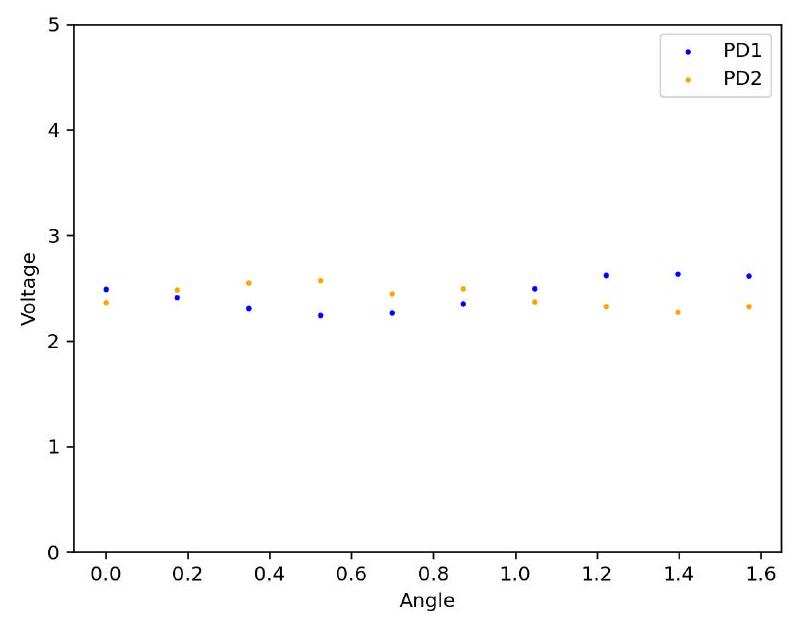
FIG. 4. Transmitted intensity of rotated HWP with incident circularly polarized light.
图4. 入射圆偏振光通过旋转半波片(HWP)的透射光强。
For a rotating QWP after circularly polarized light, following a similar calculation
对于圆偏振光后的旋转四分之一波片(QWP),进行类似的计算
such that the intensities at each photodetector are proportional to and which agree quite well with experimental results, see figure 5 .
因此每个光电探测器处的光强与 和 成正比,这与实验结果非常吻合,见图5。
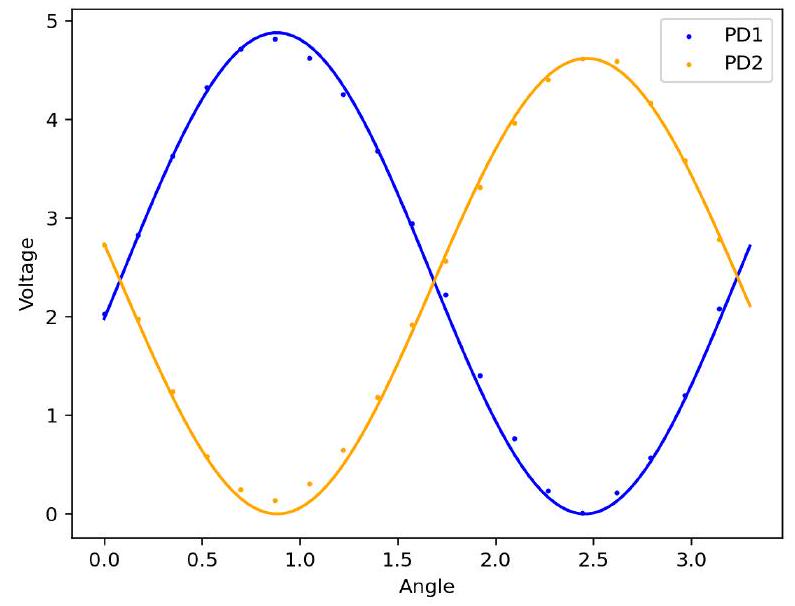
FIG. 5. Transmitted intensity of a rotated QWP with circularly polarized light incident light. The experimental data for PD1 (blue) is fit to and for PD2 (orange).
图5. 入射圆偏振光通过旋转四分之一波片(QWP)的透射光强。光电探测器1(PD1)(蓝色)的实验数据拟合为,光电探测器2(PD2)(橙色)拟合为。
We saw in the discussion above that QWPs can be used to generate circular polarization, but this is a unique case. In general, QWPs can transform linearly polarized light into what is known as elliptically polarized light in which the polarization follows an elliptical pattern as it propagates. To explore this in detail, we rotated the QWP generating circular polarization an additional 20 degrees such that it now generates elliptical polarization. Inserting a HWP between the elliptically polarized beam and the final beam splitter, the intensities at each photodiode can be shown to be
我们在上面的讨论中看到四分之一波片(QWP)可用于产生圆偏振,但这是一个特殊的情况。一般来说,四分之一波片可以将线性偏振光转换为所谓的椭圆偏振光,其中偏振在传播过程中遵循椭圆模式。为了详细探究这一点,我们将产生圆偏振的四分之一波片额外旋转20度,使其现在产生椭圆偏振。在椭圆偏振光束和最终分束器之间插入半波片(HWP),每个光电二极管处的光强可以表示为
using where and are the angles of the fast axis of the HWP and QWP from the vertical respectively. From figure 6, we see that the experimental results agree quite nicely with the theoretical model. Comparing to figures 2 and 4 , the oscillation of intensities are quite similar when linearly polarized, circularly polarized and ellipitically polarized light are sent through a rotating HWP. As the polarization changes from linear to elliptical to circular, the range of voltages decreases from and respectively. We can understand this difference conceptually as the ratio of horizontal and vertical polarization amplitudes gradually increasing to 1 as ellipticity decreases. That is, the final horizontal and vertical polarization amplitudes for an incident circularly polarized beam after it propagates through a HWP are roughly the same regardless of rotation angle since the magnitude of points along the circle are the same. However, as ellipicity increases we begin to see a larger range of voltages and ultimately the full range voltage for horizontally polarized light.
使用,其中和分别是半波片(HWP)和四分之一波片(QWP)的快轴相对于垂直方向的角度。从图6可以看出,实验结果与理论模型非常吻合。与图2和图4相比,当线性偏振、圆偏振和椭圆偏振光通过旋转半波片时,光强的振荡非常相似。随着偏振从线性到椭圆再到圆形的变化,电压的范围分别从和减小。我们可以从概念上理解这种差异,即随着椭圆率的减小,水平和垂直偏振幅度的比率逐渐增加到1。也就是说,入射圆偏振光束通过半波片传播后的最终水平和垂直偏振幅度大致相同,无论旋转角度如何,因为圆上点的幅度是相同的。然而,随着椭圆率的增加,我们开始看到更大范围的电压,最终对于水平偏振光达到完整的电压范围。
F. Generation of Arbitrary Polarization任意偏振的产生
We saw from the results and discussion above that HWPs and QWPs can be used to generate arbitrary linear and elliptical polarization respectively. We will now show that they can be used to generate arbitrary polarizations when used together. Suppose we wish to generate a polarized beam with ellipiticty that is rotated by angle with respect to the lab frame given an initially horizontally polarized beam. We will first send the beam through a HWP to create the correct horizontal and vertical polarization ratios and . The resulting Jones vector after the HWP will be
我们从上面的结果和讨论中看到半波片(HWP)和四分之一波片(QWP)分别可用于产生任意线性和椭圆偏振。现在我们将展示它们一起使用时可以产生任意偏振。假设我们希望产生一个椭圆率为并相对于实验室坐标系旋转角度的偏振光束,给定一个初始水平偏振光束。我们将首先让光束通过半波片来创建正确的水平和垂直偏振比率和。半波片后的结果琼斯矢量将是
Now we want the final beam to have an ellipiticity of such that and . To achieve
现在我们希望最终的光束具有椭圆率,使得和。为了实现这一点
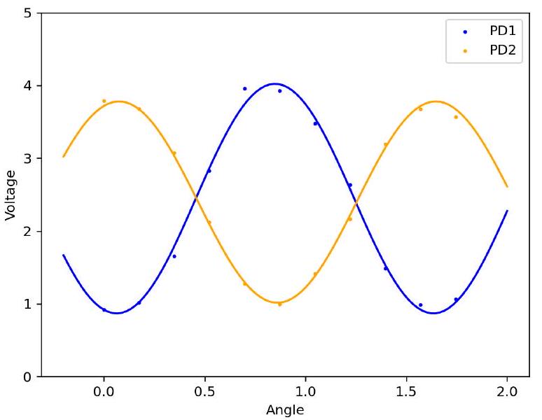
FIG. 6. Transmitted intensity of rotated HWP with elliptically polarized incident light generated with horizontally polarized incident to initial QWP with fast axis rotated 20 degrees. Experimental data for PD1 (blue) is fit to and for PD2 (orange).
图6. 旋转半波片(HWP)的透射光强,入射为椭圆偏振光,该光由水平偏振光入射到快轴旋转20度的初始四分之一波片(QWP)产生。光电探测器1(PD1)(蓝色)的实验数据拟合为 ,光电探测器2(PD2)(橙色)拟合为 。
this, we need to rotate the HWP to an angle such that . Solving for , we find that .
我们需要将半波片(HWP)旋转到角度,使得。求解,我们得到。
Now that we have the correct and ratios, we want to introduce a relative phase of between the horizontal and vertical polarization amplitudes to generate an ellipitical polarization with ellipicity . To introduce this phase shift, the beam is sent through the QWP with fast axis along the vertical such that the Jones vector is now
现在我们有了正确的和比率,我们想在水平和垂直偏振幅度之间引入的相对相位,以产生椭圆率为的椭圆偏振。为了引入这个相移,光束通过快轴沿垂直方向的四分之一波片(QWP),使得琼斯矢量现在为
and we have generated a beam with the correct ellipicity. Now to get the beam into the correct orientation in the lab frame, recall it should be rotated by angle , we want to rotate the HWP and QWP. Since rotations affect HWPs by a factor of 2, note the dependence, we will apply an additional rotation on the HWP so that its now oriented with angle from the vertical. Now if we rotate the QWP by angle , we will have successfully rotated our elliptical polarization to the desired orientation.
我们已经产生了具有正确椭圆率的光束。现在为了使光束在实验室坐标系中具有正确的取向,回想它应该旋转角度,我们需要旋转半波片(HWP)和四分之一波片(QWP)。由于旋转对半波片的影响是2的因子,注意的依赖性,我们将在半波片上施加额外的旋转,使其现在相对于垂直方向的角度为。现在如果我们将四分之一波片旋转角度,我们将成功地将椭圆偏振旋转到所需的取向。
To verify this experimentally, suppose we wanted to create a beam with ellipiticty .25 that is rotated 45 degrees in the lab frame. From our discussion above, this can be accomplished by sending a horizontally polarized beam first through a HWP rotated by angle and then through a QWP rotated by angle . To verify that we have created the desired polarization, we send the beam through a PBS and measure the horizontal and vertical polarization amplitudes using photodetectors.
为了实验验证这一点,假设我们想创建一个在实验室坐标系中旋转45度且椭圆率为.25的光束。根据我们上面的讨论,这可以通过首先将水平偏振光束通过旋转角度为的半波片(HWP),然后通过旋转角度为的四分之一波片(QWP)来实现。为了验证我们已经创建了所需的偏振,我们将光束通过偏振分束器(PBS),并使用光电探测器测量水平和垂直偏振幅度。
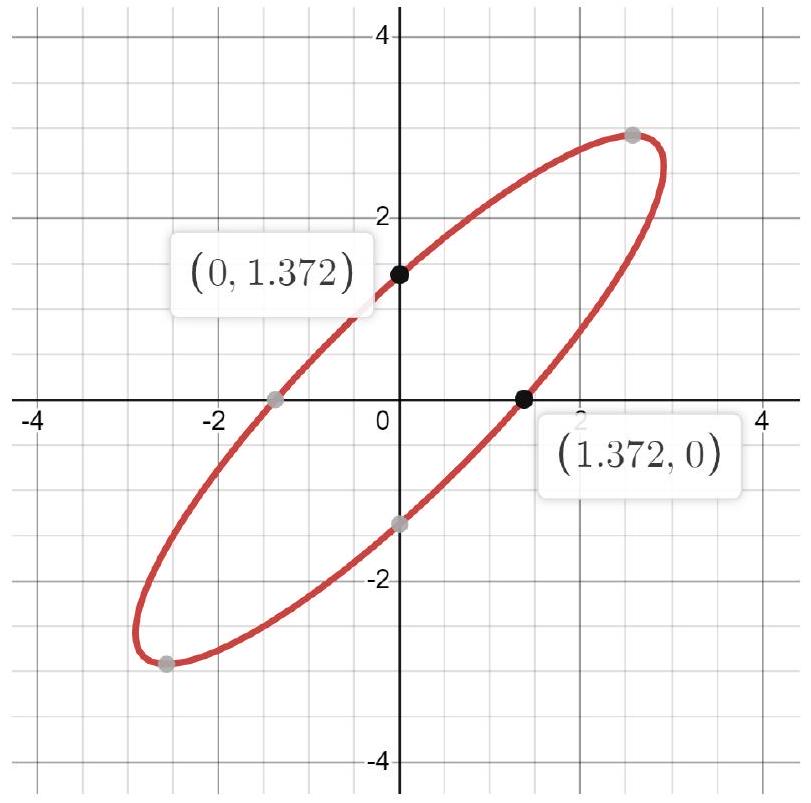
FIG. 7. Ellipse with ellipiticty .25 rotated by 45 degrees. From the figure above and from the equation for an ellipse of ellipicity .25 rotated by angle
图7. 椭圆,椭圆率为0.25,旋转45度。 从上面的图和椭圆率为0.25且旋转角度为的椭圆方程
we see that the values of the x and y intercepts are the same. Since the photodetectors at the outputs of the final PBS measure the horizontal and vertical amplitudes, we expect them to be the same for our beam. Indeed, we measured intensities of 2.429 and 2.374 volts at each photodetector. Now to verify that we have indeed created an ellipitcally polarized beam rotated at 45 degrees rather than a circularly polarized beam, we replaced the final PBS with just a linear polarizer and measured the transmitted intensities at various angles. The results are shown below
我们可以看到x和y截距的值是相同的。由于最终偏振分束器(PBS)的输出端的光电探测器测量水平和垂直振幅,我们预期它们对于我们的光束应该是相同的。确实,我们在每个光电探测器处测量到的光强分别为2.429和2.374伏特。现在为了验证我们确实创建了旋转45度的椭圆偏振光束而不是圆偏振光束,我们用一个线性偏振器替换了最终的PBS,并测量了在不同角度下的透射光强。结果如下所示
As we expect, the intensity is maximized when the polarizer is rotated from the horizontal since the magnitude of points along the rotated ellipse is maximal at 45 and (225) degrees.
正如我们预期的,当偏振器从水平方向旋转时,光强达到最大值,因为沿着旋转椭圆的点的幅度在45和(225)度处达到最大。
G. Optical Isolator****光学隔离器
When working with optics, it is often important to avoid reflecting the beam in the system back into the laser source as this produces unwanted intensities in the system. To resolve this issue we can implement what is known as an optical isolator with just a QWP. Consider the setup in which we send a laser source through a PBS with a QWP and silvered mirror in the orthogonal
在使用光学系统时,避免将系统中的光束反射回激光源通常很重要,因为这会在系统中产生不需要的光强。为了解决这个问题,我们可以仅用一个四分之一波片(QWP)实现所谓的光学隔离器。考虑这样一个装置:我们将激光源通过一个偏振分束器(PBS)发送,在正交
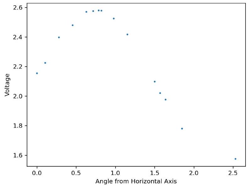
FIG. 8. Transmitted intensity of a rotated linear polarizer incident with ellipitically polarized light rotated by 45 degrees with ellipicity .25. output arm of the split beams. We can treat silvered mirror as the optical system which reflects some unwanted light back into the laser source. To get a sense of how much of the reflected beam goes back into the laser, we will measure the intensity of the beam on the side of the PBS that is opposite from the QWP and mirror. Note that high intensities measured by the photodetector here means the beam is sent to the photodetector and not the laser source, which is the intended purpose of the optical isolator. Experimental results of this setup is shown below as the QWP is rotated
图8. 旋转线性偏振器的透射光强,入射为旋转45度且椭圆率为0.25的椭圆偏振光。 分离光束的输出臂。我们可以将镀银镜视为光学系统,它将一些不需要的光反射回激光源。为了获得反射光束返回激光器的多少的感知,我们将测量偏振分束器(PBS)上与四分之一波片(QWP)和镜子相对的一侧的光束的光强。注意,这里由光电探测器测量到的高光强意味着光束被发送到光电探测器而不是激光源,这正是光学隔离器的预期目的。下图显示了当四分之一波片旋转时该装置的实验结果
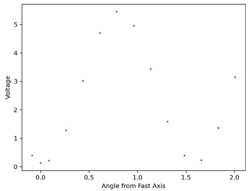
FIG. 9. Transmitted light in optical isolator system away from laser source.
图9. 光学隔离器系统中远离激光源的透射光。
When the QWP is rotated such that the fast axis is from the vertical, the beam is sent entirely into the photodetector and nothing gets reflected back into the laser source.
当四分之一波片(QWP)旋转使其快轴与垂直方向成角时,光束完全被发送到光电探测器,没有任何东西被反射回激光源。
To understand this conceptually, we can think of the PBS as an optical device that only transmits horizontally polarized light to and from the laser source while vertically polarized light is transmitted away from the laser (in this case toward this photodetector). In practice, this can be implemented with just a horizontal polarizer. Now the beam that first enters the QWP is purely horizontally polarized. If the QWP is rotated such that its fast axis is 45 degrees from the vertical, we saw from the discussion above that this generates circularly polarized light. After the circularly polarized light is reflected from the silvered mirror, the polarization changes what is known as helicity or handedness. Conceptually, helicity is the 'direction' in which the circularly polarized beam rotates. Circularly polarized light can either be left or right circularly polarized depending on its helicity. Mathematically, it is just a phase shift of . After the beam changes helicity, it will again propagate through the QWP but this time the beam is transformed so that the polarization is entirely vertical due to the difference in helicity. To verify this claim, readers may perform a similar derivation to equation 19 with a vertically polarized beam and find that the resulting Jones vector is identical expect for a phase shift of such that circularly polarized light with a different helicity is produced. Going back to the system, now that the returning beam is vertically polarized, none of the light is reflected back into the laser source and instead we measure the full beam at the photodetector! Using just a linear polarizer and QWP, we have created an optical isolator that prevents reflected beams going back into the laser source.
从概念上理解这一点,我们可以将偏振分束器(PBS)视为一种只允许水平偏振光往返于激光源的光学装置,而垂直偏振光则被传输离开激光器(在这种情况下朝向光电探测器)。在实践中,这可以仅用一个水平偏振器来实现。现在,首先进入四分之一波片(QWP)的光束是纯水平偏振的。如果四分之一波片旋转使其快轴与垂直方向成45度角,我们从上面的讨论中看到这会产生圆偏振光。当圆偏振光从镀银镜反射后,偏振改变了所谓的螺旋度或手性。从概念上讲,螺旋度是圆偏振光束旋转的"方向"。圆偏振光可以是左旋或右旋圆偏振,取决于其螺旋度。从数学上讲,这只是的相移。在光束改变螺旋度后,它将再次通过四分之一波片传播,但这次由于螺旋度的差异,光束被转换为完全垂直的偏振。为了验证这一说法,读者可以对垂直偏振光束执行类似于方程19的推导,并发现所得的琼斯矢量除了的相移外是相同的,从而产生具有不同螺旋度的圆偏振光。回到系统,现在返回的光束是垂直偏振的,没有光被反射回激光源,相反,我们在光电探测器处测量到完整的光束!仅使用线性偏振器和四分之一波片,我们创建了一个光学隔离器,防止反射光束返回激光源。
The careful reader will notice that this optical isolator only works if the reflected beam from the system is circularly polarized with opposite helicity from the incoming beam. If the system produces reflected beams that have a different polarization, the optical isolator will not work as effectively (or at all if the reflected beam is circularly polarized with the same helicity). Additionally, this optical isolator with the initial horizontal polarizer reduces the beam intensity by a half if the laser source produces unpolarized light. While this optical isolator works in certain cases, it effectively trades cost for practicality.
细心的读者会注意到,这种光学隔离器只有在系统反射的光束是与入射光束具有相反螺旋度的圆偏振光时才有效。如果系统产生具有不同偏振的反射光束,光学隔离器将不会那么有效(如果反射光束是具有相同螺旋度的圆偏振光,则完全无效)。此外,如果激光源产生非偏振光,这种带有初始水平偏振器的光学隔离器会将光束强度减半。虽然这种光学隔离器在某些情况下有效,但它实际上是用成本换取实用性。
III. SPONTANEOUS PARAMETRIC DOWN-CONVERSION III. 自发参量下转换
Now that we have a good understanding of polarizations and its transformation through optical elements, let us explore the nature of light and whether quantum mechanics is a good formalism to explain its behavior. In particular, we will explore maximally entangled photon pairs that can be generated in a process known as Spontaneous Parametric Down-Conversion (SPDC). The idea behind SPDC is to convert a single high energy photon into a lower energy photon pair. This can be done via a non-linear optical element known as a non-linear crystal. The details of how a non-linear crystal operates requires an understanding of non-linear optics and is outside the scope of this paper, but fundamentally a non-linear crystal can convert a high energy, linearly polarized photon into a pair of lower energy photons polarized in an orthogonal axis with very low probability (typically ). For instance, an incoming horizontally polarized blue photon can emerge from a non-linear crystal as a pair of vertically polarized red photons. Energy and momentum conservation requires that the non-linear crystal converts an incident photon with energy to a pair of photons with energies in a cone-like emission pattern with photon pairs at opposite ends of the cone, see figure 10. The opening angle of the emission cone depends on the wavelength of the pump photons in accordance to energy and momentum conservation.
现在我们对偏振及其通过光学元件的转换有了很好的理解,让我们探索光的本质以及量子力学是否是解释其行为的良好形式。特别地,我们将探索可以通过称为自发参量下转换(SPDC)的过程产生的最大纠缠光子对。SPDC背后的理念是将单个高能光子转换为低能光子对。这可以通过被称为非线性晶体的非线性光学元件来实现。关于非线性晶体如何运作的细节需要理解非线性光学,这超出了本文的范围,但从根本上讲,非线性晶体可以将高能、线性偏振的光子转换为一对在正交轴上偏振的低能光子,但概率非常低(通常为)。例如,一个入射的水平偏振蓝色光子可以从非线性晶体中出现为一对垂直偏振的红色光子。能量和动量守恒要求非线性晶体将具有能量的入射光子转换为一对具有能量的光子,形成锥状发射模式,光子对位于锥体的相对两端,见图10。发射锥的开口角度取决于泵浦光子的波长,符合能量和动量守恒。
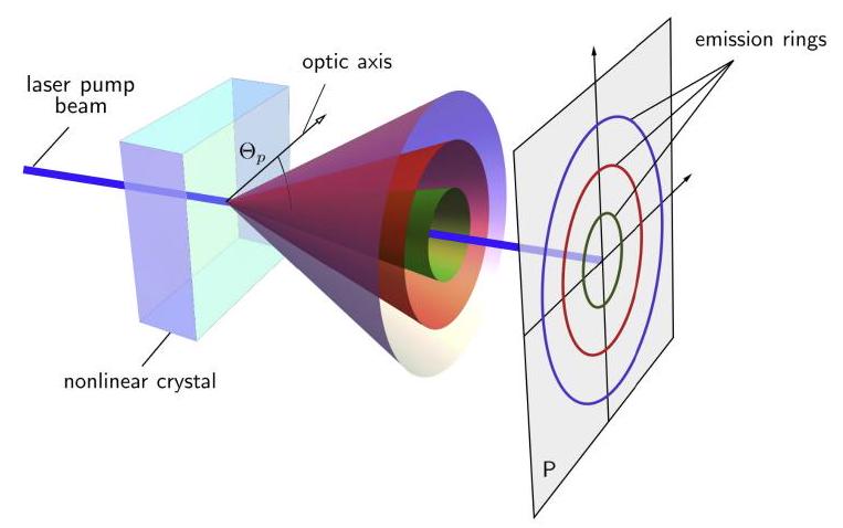
FIG. 10. Spontaneous parametric down-conversion via nonlinear crystal. The SPDC photons follow a cone-like emission pattern whose opening angle depends on the wavelength of pump photons.
图10. 通过非线性晶体的自发参量下转换。SPDC光子遵循锥状发射模式,其开口角度取决于泵浦光子的波长。
To produce entangled photon pairs using SPDC, consider a pair of non-linear crystals oriented such that their optical axes are mutually orthogonal. For instance, suppose the optical axis of the first (second) crystal is aligned to the horizontal (vertical) plane. In this setup in particular, incoming horizontally (vertically) polarized photons can be down-converted only in the first (second) nonlinear crystal, transforming into a pair of vertically (horizontally) polarized photons. Now suppose that the pump photons are diagonally polarized at 45 degrees from the horizontal. This can be realized with a linear polarizer at 45 degrees for unpolarized pump photons or with a HWP with fast axis rotated 22.5 degrees from the vertical for horizontally polarized pump photons. By pumping the crystals with diagonally polarized light, there is an equal probability that the photons are down-converted in either crystal. Provided there is no way of determining whether the down-conversion occurred in the first or second crystal, the resulting SPDC photon pairs are in the entangled state
要使用SPDC产生纠缠光子对,考虑一对非线性晶体,它们的光轴相互正交。例如,假设第一(第二)晶体的光轴分别与水平(垂直)平面对齐。在这个特定的装置中,入射的水平(垂直)偏振光子只能在第一(第二)非线性晶体中下转换,转变为一对垂直(水平)偏振的光子。现在假设泵浦光子相对于水平方向呈对角线偏振45度。这可以通过对未偏振泵浦光子使用45度的线性偏振器来实现,或者对水平偏振泵浦光子使用快轴从垂直方向旋转22.5度的半波片(HWP)来实现。通过用对角线偏振光泵浦晶体,光子在任一晶体中下转换的概率相等。如果无法确定下转换发生在第一还是第二个晶体中,则产生的SPDC光子对处于纠缠态
where the relative phase can be controlled by adjusting the relative phase between the horizontal and vertical components, and , of the pump photons.
其中相对相位可以通过调整泵浦光子的水平和垂直分量和之间的相对相位来控制。
In particular, the entangled state is generated with anti-diagonally polarized light while is generated with diagonally polarized light.
特别地,纠缠态是用反对角线偏振光产生的,而是用对角线偏振光产生的。
A. Apparatus装置
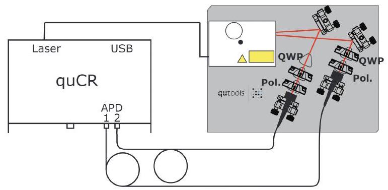
FIG. 11. quED apparatus. The laser source (white rectangle in upper right) generates SPDC photon pairs in state that are redirected using mirrors through QWPs and linear polarizers into an optical fiber for coincidence measurements at the quCR.
图11. quED装置。激光源(右上角的白色矩形)产生处于态的SPDC光子对,这些光子对通过镜子重定向,经过QWP和线性偏振器进入光纤,在quCR进行符合测量。
The device used in our entanglement experiments will be referred to as the quED (quantum entanglement demonstrator) and a diagram of the apparatus is shown in figure 11. The laser source generates entangled photon pairs following the discussion of above with a HWP to produce diagonally polarized light and a pair of nonlinear crystals for SPDC along with additional corrective elements to maximize the entanglement quality. The cone-like emission pattern of the entangled photon pairs are redirected using a pair of silvered mirrors into optical fibers which can then be registered as coincidence counts using the quCR (Control and Readout unit) which detects coincidences at a time interval of 20 ns . It is crucial that the optical path length of the two arms are near identical so that coincidences can be detected and measured correctly.
我们的纠缠实验中使用的设备被称为quED(量子纠缠演示器),装置的图示如图11所示。激光源按照上述讨论生成纠缠光子对,使用半波片(HWP)产生对角线偏振光和一对用于SPDC的非线性晶体,以及额外的校正元件以最大化纠缠质量。纠缠光子对的锥状发射模式通过一对镀银镜子重定向到光纤中,然后可以使用quCR(控制和读出单元)记录为符合计数,该单元在20纳秒的时间间隔内检测符合。两个臂的光路长度几乎相同是至关重要的,这样才能正确地检测和测量符合。
The laser source operates by sending a continuous source of pump photons proportional to its pump current. Since the rate of SPDC in the non-linear crystals depend only on the properties of the crystal, we expect that the number of SPDC photon pairs grows proportionally to the pump current. Indeed, after optimizing the alignment of the mirrors and fiber optic cables in each arm to maximize the coincidence rates, we find that the number of coincidence counts grows linearly with pump power in figure 12.
激光源通过发送与其泵浦电流成比例的连续泵浦光子****源来运行。由于非线性晶体中SPDC的速率仅取决于晶体的特性,我们预期SPDC光子对的数量与泵浦电流成比例增长。确实,在优化每个臂中镜子和光纤电缆的对准以最大化符合率后,我们发现符合计数的数量与泵浦功率呈线性增长,如图12所示。
The quED laser source has a maximum pump current of 10 mW . As we begin to saturate this maximum threshold, the coincidence rate to power ratio starts to taper off in figure 12 since the actual current is slightly lower than
quED激光源的最大泵浦电流为10 mW。当我们开始接近这个最大阈值时,符合率与功率比开始在图12中趋于平缓,因为实际电流略低于
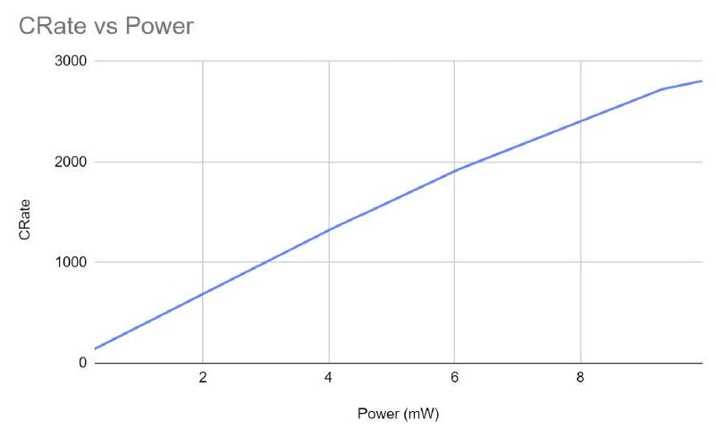
FIG. 12. Coincidence count rate as a function of laser power.
图12. 符合 计数 率随激光 功率的函数关系。
| Basis | Avg | |||||
|---|---|---|---|---|---|---|
| HH | 2682 | 2712 | 2655 | 2699 | 2651 | 2679.8 |
| VV | 1731 | 1803 | 1760 | 1780 | 1762 | 1767.2 |
| HV | 82 | 86 | 66 | 79 | 104 | 83.4 |
| VH | 81 | 94 | 95 | 88 | 93 | 90.2 |
| PM | 307 | 327 | 336 | 304 | 317 | 318.2 |
| MP | 329 | 277 | 285 | 328 | 326 | 309 |
| PP | 2092 | 1942 | 1927 | 2068 | 1935 | 1992.8 |
| MM | 1842 | 1908 | 1837 | 1800 | 1840 | 1845.4 |
TABLE I. Coincidence counts of measurements in various polarization bases.
表 I. 各种 偏振 基的测量 符合 计数。
B. Visibility and Entanglement Quality B. 可见性和纠缠 质量
The quED device is now set-up to produce pairs of entangled down-converted photons that are roughly in the triplet state . Before taking experimental data, it is helpful to first gauge the entanglement quality of these photons since it affects how well experimental results agree with theory. For instance, highly entangled photon pairs that are close to the triplet state will produce experimental data that is close to theoretical predictions.
quED 设备现在设置为产生 纠缠 下转换 光子 对,它们大致处于三重态 。在 获取 实验 数据 之前,首先 评估这些光子的纠缠 质量是有帮助的,因为它影响 实验 结果与理论的一致性。例如,高度 纠缠的光子 对 接近 三重态 将产生 接近 理论 预测的实验 数据。
The data in table I contain the coincidence counts with the arms of the quED apparatus set at various polarization bases. The angles of the QWP and polarizers used to project onto the different polarization bases are given in table II. For instance, if we wish to generate diagonally polarized light, , from unpolarized light using a polarizer and QWP we could do so by rotating the polarizer and QWP to . The polarizer filters the unpolarized light so that only diagonally polarized light leaves. The QWP does nothing since its optical axis is aligned with the incoming polarization. See the discussion on Jones calculus above as necessary. Now to project onto the basis, we could imagine applying the polarizer and QWP in the reverse order as in figure 11.
表 I 中的数据 包含 quED 装置的臂在各种 偏振 基上的符合 计数。用于 投影到不同 偏振 基的QWP和偏振器的角度在表 II 中给出。例如,如果我们希望 生成 对角线 偏振 光 ,从未偏振 光 使用 偏振器和QWP,我们可以通过将偏振器和QWP旋转到 来实现。偏振器 过滤 未偏振 光,使得 只有 对角线 偏振 光 离开。QWP 不做任何事情,因为其光轴与入射 偏振 对齐。必要时,请参阅上面关于琼斯 算法的讨论。现在,为了投影到 基,我们可以想象 反向 应用 偏振器和QWP,如图 11 所示。
Since we are generating entangled photon pairs in the triplet state
由于我们正在生成 三重态的纠缠 光子 对
we expect that the coincidence counts are high and roughly the same. Indeed, we see from the data in I that the coincidences of are high whereas those of the other basis states HV,VH,PM,MP are low. Unfortunately, due to imperfect alignment there are slightly more HH coincidences than VV coincidences so that the quED apparatus produces entangled photon pairs that are close to but not exactly the triplet state . To neatly characterize the entanglement quality, let us define the visibility as
我们期望 的符合 计数 高且大致相同。确实,我们从 I 中的数据看到 的符合 高,而其他 基 态 HV,VH,PM,MP 的符合 低。不幸的是,由于 对准 不完美,HH 的符合 略多于 VV 的符合,因此 quED 装置 产生的纠缠 光子 对 接近 但不完全是 三重态 。为了 整齐地 表征 纠缠 质量,让我们 定义 可见性为
where is the maximum and minimum coincidence counts respectively for a chosen basis. For a perfectly generated triplet state , there would only be coincidence measurements in the HH,VV,PP and MM bases and all other bases would have a coincidence count of 0 for a maximum visibility of 1 . Due to imperfect alignment, stray beams, dark counts, etc the quED apparatus does not generate perfect triplet states and we instead find that
其中 分别是 选定 基的最大和最小 符合 计数。对于 完美生成的三重态 ,只有在 HH,VV,PP 和 MM 基中有 符合 测量,所有 其他 基的符合 计数为 0,最大 可见性为 1。由于 对准 不完美、杂散 光束、暗 计数等,quED 装置 未能 生成 完美的三重态 ,我们 发现
and 和
which is not optimal but sufficient for the purposes of this lab. These results, thus far, do not rule out the existence of a local hidden variable theory in which some hidden variable may exist with photons that can be used to compute polarization measurements without doing the measurement. The local hidden variable theory will be discussed thoroughly in section VI.
这 不是 最佳的,但 足以 满足本实验的目的。这些 结果 到目前为止 并未 排除 局域 隐变量 理论的存在,其中 可能 存在 一些 隐变量 与 光子 一起,可以 用于 计算 偏振 测量 而不 进行 测量。局域 隐变量 理论 将在 第 VI 节 中 详细讨论。
IV. QUANTUM STATE TOMOGRAPHY IV. 量子 态 层析
Using our quED apparatus, we can perform what is known as quantum state tomography to reconstruct the density matrix of a system where
使用我们的quED 装置,我们 可以 执行 所谓的 量子 态 层析,以重建 系统的密度 矩阵 ,其中
| Projection | QWP Polarizer | Measured Quantity | |
|---|---|---|---|
TABLE II. Various projection bases produced by QWP and linear polarizer at respective angles.
表 II. 由 QWP 和 线性 偏振器在各自 角度 产生的各种 投影 基。
and is the probability of producing state in the system. For our quED system in particular, we are (ideally) always producing the triplet state such that the density matrix of the system is
和**是系统中产生态** 的概率。特别是对于我们的quED 系统,我们(理想情况下)总是产生三重态 ,使得系统的密度矩阵为
We can also take the partial trace of a multi-qubit system to find the density matrix of only a portion of the system. Here the partial trace of system A in composite system AB is defined as
我们还可以对多量子比特系统进行部分迹,以找到系统中某一部分的密度矩阵。这里复合系统AB中系统A的部分迹定义为
For our quED system, taking the partial trace of 33 we find that the density matrix of a single qubit state is
对于我们的quED系统,对33进行部分迹,我们发现单量子比特态的密度矩阵为
To perform quantum state tomography using our quED setup and coincidence counts, we use linear inversion to express the density matrix for an n qubit system as
为了使用我们的quED设置和符合计数进行量子态层析,我们使用线性反演来表示n量子比特系统的密度矩阵为
where , are the Pauli matrices and the correlation tensor T is given by
其中**** ,是泡利矩阵,关联张量 T由下式给出
for and . Here are the coincidence counts for the basis , is the total coincidence counts for that basis and g is a parity function that determines the sign of the contribution. For instance, for two qubit tomography we can express
对于**和。这里是基的符合计数**,是该基的总符合计数,g是确定贡献的符号的奇偶函数。例如,对于双量子比特层析,我们可以表示为
and
以及
according to the grouping of bases and .
根据基**和的分组**。
In particular, single qubit tomography requires 6 measurements in the and basis with the density matrix expressed as
特别是,单量子比特层析需要在**和基中进行6次测量**,其密度矩阵表示为
for . Using the single qubit tomography data in table III, we find that the density matrix is
对于**。使用表III中的单量子比特层析数据**,我们发现密度矩阵为
which is quite close to the theoretical prediction in equation 35. We see the effects of the imperfect triplet state generation here as the component is slightly larger than the component in accordance with more HH coincidences than VV coincidences in table I.
这与方程35中的理论预测非常接近。我们看到这里不完美的三重态生成的影响,因为**** 分量略大于**** 分量,这与表I中的HH符合多于VV符合一致。
Two qubit tomography, requires basis measurements for each qubit in the and L basis. Following a similar procedure outlined above and using two qubit tomography data in table IV, we find that the density matrix is
双量子比特层析需要在**和L基中对每个量子比特进行基测量**。按照上面概述的类似步骤并使用表IV中的双量子比特层析数据,我们发现密度矩阵为
Again, we see that the two qubit density matrix is quite close to the theoretical prediction in equation 33. The and contributions in each corner of the density matrix are dominant with a higher amplitude in the component due to the higher coincidence counts in the HH basis. With better alignment and higher visibility, the amplitudes would be better distribution in the four corners of the density matrix.
再次,我们看到双量子比特密度矩阵与方程33中的理论预测非常接近。密度矩阵的每个角落中的**和贡献是显著的,因为HH基中的符合计数较高,导致** 分量的幅度较高。通过更好的对准和更高的可见性,幅度将在密度矩阵的四个角落中更好地分布。
| Basis | Counts |
|---|---|
| H | 45371 |
| V | 40908 |
| P | 37581 |
| M | 39850 |
| R | 34673 |
| L | 38232 |
TABLE III. Single counts in respective projection basis. Data used for single qubit tomography.
表 III. 各自投影基中的单次计数。用于单量子比特层析的数据。
| basis | H | V | P | M | R | L |
|---|---|---|---|---|---|---|
| H | 1325 | 41 | 762 | 714 | 602 | 806 |
| V | 37 | 762 | 347 | 391 | 384 | 352 |
| P | 547 | 419 | 990 | 120 | 303 | 738 |
| M | 602 | 354 | 138 | 890 | 63 | 332 |
| R | 462 | 409 | 34 | 673 | 84 | 899 |
| L | 624 | 367 | 782 | 313 | 847 | 189 |
TABLE IV. Coincidence counts at various pairs of basis projections. Data is used for two qubit tomography.
表 IV. 各种基投影对的符合计数。用于双量子比特层析的数据。
V. NATURE OF LIGHT****光的本质
Ever since the mid 19th century, Maxwell's equations theorized that light is an electromagnetic field that can take on any field energy. For the most part, this interpretation of light and a continuous energy field has agreed well with experiments and theories, holding up to even Einstein's theory of general relativity. In the early 20th century, however, quantum mechanics predicts that light only exists in quantized energy packets known as photons which cannot be split into smaller packets.
自19世纪中期以来,麦克斯韦方程理论化了光是一种可以承载任何场能量的电磁场。在大多数情况下,这种对光和连续能量场的解释与实验和理论非常吻合,甚至与爱因斯坦的广义相对论理论相符。然而,在20世纪初,量子力学预测光仅以称为光子的量化能量包存在,不能分割成更小的包。
To explore the nature of light and determine whether a classical or quantized approach serves as a better interpretation, consider the modified quED apparatus in figure 13 in which an additional (in wire) beamsplitter is inserted into one arm and all three outputs are measured using a coincidence counter. Our actual experiment set up the connections differently such that channels are referred to respectively in our data. For the moment, let us only consider the arm with the beamsplitter and ignore the process occurring in the other arm that connects to channel 0 in the figure. We can imagine that the laser is a continuous single photon source that sends a beam of photons into a BS before their coincidence counts are measured by a detector. If light behaves as a
为了探索光的本质并确定经典或量化方法是否作为更好的解释,请考虑图13中的修改后的quED装置,其中一个臂中插入了额外的(在线)分束器,并使用符合计数器测量所有三个输出。我们的实际实验设置了不同的连接,使得通道 在我们的数据中分别称为**。目前,让我们只考虑带有分束器的臂**,忽略连接到图中通道0的另一个臂中发生的过程。我们可以想象激光器是一个连续单光子源,在其符合计数由探测器测量之前,将光子束发送到BS。如果光表现为
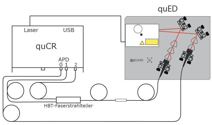
FIG. 13. quED with an additional herald/control arm connected to channel 0. In the other arm, photons are split via an in wire polarizing beam splitter before they are detected at channels 1 and 2.
图13. quED装置,带有连接到通道0的额外信号/控制臂。在另一个臂中,光子通过内置线偏振分束器分离,然后在通道1和2处被探测。
continuous field in the classical regime, we should expect that the 5050 BS would split incoming photons into two lower energy pairs that would be detected as a single coincidence. On the other hand, if light were to behave as a quantized wavepacket that cannot be split into smaller packets, the photon would travel entirely into one arm of the BS so that no coincidences would be detected. See figure 14 for a graphical representation.
在经典区域中的连续场,我们应该预期5050分束器(BS)会将入射光子分成两对较低能量对,这将被检测为单个符合计数。另一方面,如果光表现为不能分裂成更小数据包的量子波包,光子将完全进入分束器(BS)的一个臂,因此不会检测到符合计数。参见图14的图形表示。

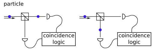
FIG. 14. Right: Coincidence logic unit registers a coincidence count for a wave-like photon split evenly by the PBS. Center and left: Coincidence logic unit does not register a coincidence since photon travels in one or the other path (but not both simultaneously).
图14. 右图:符合逻辑单元为被偏振分束器(PBS)均匀分割的波状光子记录符合计数。中间和左图:符合逻辑单元不记录符合,因为光子仅在一条路径中传播(而不是同时在两条路径中)。
We can characterize the normalized correlations using the second order correlation function as a function of probabilities:
我们可以使用二阶关联函数 作为概率的函数来表征归一化关联:
where is the probability to detect an event at detectors 1 and 2 respectively and is the probability of making a detection in both detectors in the same time interval. Since we will be working with discrete counts rather than probabilities, we can re-express the correlation function using such that
其中分别是在探测器1和2处检测到事件的概率,是在相同时间间隔内在两个探测器中进行检测的概率。由于我们将使用离散计数而不是概率,我们可以使用重新表示关联函数,使得
is the count at detector(s) i and is the coincidence time interval in seconds. Before we compute the experimental value of , let us first take a moment to understand how to interpret the values. When individual photons are measured such that no photons are detected directly following one another, we should expect that there will be minimal coincidence counts and and thus will be close to 0. On the other hand, when either the source produces purely random photon emissions such that we cannot guarantee single photon measurements or if light follows a classical wavelike picture, there will be coincidence counts for virtually all photons such that will be at or above 1. Using the coincidence data listed in table V with a coincidence time interval of , we find that
是探测器i处的计数,是以秒为单位的符合时间间隔。在我们计算的实验值之前,让我们先花片刻时间了解如何解释这些值。当测量单个光子时,如果没有光子直接跟随另一个被检测到,我们应该预期会有最小的符合计数和,因此将接近0。另一方面,当源产生纯随机光子发射,使我们无法保证单光子测量,或者如果光遵循经典波状图像,几乎所有光子都会有符合计数,使达到或超过1。使用表V中列出的符合数据,符合时间间隔为,我们发现
We find experimentally that the correlation function results in a value that is greater than 1! This is the value we might expect for a laser source or photons that behave in the classical regime. Does this imply that light is composed of continuous energy fields and quantum mechanics has failed? It would if the system was set up correctly. The problem with the aforementioned setup is that we cannot treat the laser source as a single photon source. The non-linear crystals in the laser source setup converts pump photons into lower energy photons pairs at a rate of . The remaining unconverted photons will enter the BS and into the detectors in a fashion that is not a single photon source but rather a continuous stream of high energy photons. As a result, we measure a correlation function with value greater than 1 as we might expect for a continuous laser source.
我们通过实验发现关联函数的值大于1!这是我们可能对激光源或在经典区域中行为的光子预期的值。这是否意味着光由连续能量场组成,而量子力学已经失败?如果系统设置正确,确实如此。上述设置的问题是我们不能将激光源视为单个光子源。激光源设置中的非线性晶体以的速率将泵浦光子转换为较低能量光子对。剩余未转换的光子将进入分束器(BS)并进入探测器,其方式不是单个光子源,而是高能量光子的连续流。因此,我们测量到值大于1的关联函数,这正如我们对连续激光源的预期。
We can still treat the SPDC photons, however, as a single photon source since only a few thousand such photons are converted by the non-linear crystals each second. In order to measure SPDC photons in our coincidence counts rather than the higher energy pump photons, we can use the fact that SPDC photons occur in pairs to our advantage. That is, if we detect an SPDC photon in one arm we can assume with high probability that the other SPDC photon pair is in the other arm, with the exception of dark counts, stray photons, etc. Therefore, we can condition coincidence detection events using an idler or herald arm. In our quED apparatus in particular, this translates to using the arm we previously ignored (the arm that connects to channel 0 in figure 13) as a way of conditioning the coincidence counts and ensuring our measurements are taken from a single photon source. Conditioning the correlation function with respect to counts in channel 3, we can write
然而,我们仍然可以将SPDC光子视为单个光子源,因为每秒只有几千个这样的光子被非线性晶体转换。为了在我们的符合计数中测量SPDC光子而不是更高能量的泵浦光子,我们可以利用SPDC光子成对出现的事实作为我们的优势。也就是说,如果我们在一个臂中检测到SPDC光子,我们可以以高概率假设另一个SPDC光子对在另一个臂中,除了暗计数、杂散光子等例外情况。因此,我们可以使用闲置或信号臂来条件符合检测事件。特别是在我们的quED装置中,这意味着使用我们之前忽略的臂(连接到图13中通道0的臂)作为条件符合计数的方式,并确保我们的测量来自单个光子源。相对于通道3中的计数条件化关联函数,我们可以写
for the heralded second order correlation function. As before, if photons behaved as continuous energy fields, we would expect a count in all three detectors for every SPDC photon pair. Using the coincidence data from figure , we find that
对于信号二阶关联函数。如前所述,如果光子表现为连续能量场,我们预期每个SPDC光子对在所有三个探测器中都有计数。使用图中的符合数据,我们发现
which is very close to 0 . With the additional herald arm ensuring that we are close to a single photon source, we find experimental evidence that photons are quantized packets rather than classical continuous energy fields!
这非常接近0。通过额外的信号臂确保我们接近单个光子源,我们找到了实验证据表明光子是量子化的数据包而不是经典的连续能量场!
| 19097 | 20270 | 43661 | 11 | 1560 | 1760 | 2 |
| 19151 | 20460 | 44065 | 11 | 1536 | 1494 | 2 |
| 18846 | 20105 | 43799 | 14 | 1526 | 1550 | 2 |
| 18712 | 20110 | 43595 | 9 | 1599 | 1548 | 0 |
| 19010 | 20195 | 43674 | 10 | 1589 | 1549 | 0 |
| 18963.2 | 20228 | 43758.8 | 11 | 1562 | 1580.2 | 1.2 |
TABLE V. Photon counts in channel respectively. Coincidence counts in channels respectively. denotes a coincidence in all 3 channel simultaneously. HV visibility: 98.7. PM visibility: 84.4
表 V. 光子计数 分别在通道 中。符合计数 分别在通道 中。 表示所有3个通道同时的符合。HV可见度:98.7。PM可见度:84.4
VI. BELL INEQUALITY VI. 贝尔不等式
Quantum mechanics wasn't always accepted as a sound and structured theory. There have been many opponents of quantum mechanics in the early 20th century including Einstein who dismissed the theory as 'spooky action at a distance'. Physicists at the time were most uncomfortable with the notion that quantum mechanics is a probabilistic theory. There was no way of knowing basic information about a state such as its position or momentum with certainty before it was measured and thus completely going against the established understanding of physics as field that predicts the behavior of evolving systems. Rather than a probabilistic theory in which information is gained only when measurements are performed, the Local Hidden Variable theory emerged at the time with the premise that these probabilistic states instead had a classical 'hidden-variable' that predetermined information about the system even before it is measured. After all, perhaps our understanding of physics is incomplete and there exists 'hidden-variables' that we don't know about (yet) that we could use to determine information about the system.
量子力学并非一直被接受为一种合理且结构化的理论。在20世纪早期,量子力学有许多反对者,包括爱因斯坦,他将该理论称为"幽灵般的远距离作用"。当时的物理学家对量子力学是一种概率性理论的概念感到非常不适。在测量之前,无法确定地知道关于态的基本信息,如其位置或动量,这完全违背了对物理学的既定理解,即物理学作为预测演化系统行为的领域。与仅在执行测量时才获得信息的概率性理论不同,局域隐变量理论在当时出现,其前提是这些概率性态实际上具有经典的"隐变量",即使在测量之前就预先确定了关于系统的信息。毕竟,也许我们对物理学的理解是不完整的,存在着我们(尚)不知道的"隐变量",我们可以用它来确定关于系统的信息。
To explore the practicality of this local hidden variable theory, suppose we have two parties Alice and Bob that are separated sufficiently far apart and perform measurements that are sufficiently synchronized such that their measurements do not affect one another. Suppose Alice and Bob are performing a series of single measurements of photon pairs and in their own lab frames respectively where the operators
为了探索这种局域隐变量理论的实用性,假设我们有两个方,爱丽丝和鲍勃,他们相距足够远,并执行足够同步的测量,使得他们的测量不会相互影响。假设爱丽丝和鲍勃分别在自己的实验室坐标系中对光子对 和 进行一系列单一测量,其中算符
measure the polarization of the photon in the basis rotated by angle . Here is a measurement in the HH and VV basis. These operators have eigenvalues so measurements Alice and Bob perform will always result in either +1 or -1 .
测量在由角度 旋转的基中光子的偏振。这里 是在HH和VV基中的测量。这些算符具有本征值 ,因此爱丽丝和鲍勃执行的测量将始终得到+1或-1的结果。
Suppose we conduct an experiment in which we measure the expectation value of the following observable:
假设我们进行一个实验,测量以下可观测量的期望值:
Here is known as Bell's observable named after physicist John Bell. At this point it isn't clear why Bell's observable was constructed in this manner but we will soon see that this observable will resolve whether the local hidden variable theory is sufficient or whether quantum mechanics is necessary. For now, suppose Alice and Bob were to carry out this task of measuring . They would be sent photon pairs of the form
这里 被称为贝尔可观测量,以物理学家****约翰·贝尔命名。在这一点上,尚不清楚为什么贝尔可观测量以这种方式构建,但我们很快就会看到,这个可观测量将解决局域隐变量理论是否足够或者量子力学是否必要的问题。现在,假设爱丽丝和鲍勃要执行测量 的任务。他们将被发送形式为
and at random Alice and Bob would measure the photon in either the or basis which we denote their measurement results as and t respectively. Let us assume for the moment, as the local hidden variable theory suggests, that each particle carries some hidden variable that can be used to compute the measurement results of Alice and Bob before they carry out the measurement. Although we may not know what this variable exactly might be or how it affects our measurements, if we perform enough measurements by Alice and Bob we can get a distribution of their 16 results that would theoretically be averaged by the distribution governing values. Let denote the probability of outcome and t of which there are 16 possibilities. We can imagine that depends on the hidden variable that could be used to compute the results and t . Therefore, using standard statistics the expectation value of a pair of measurements done by Alice and Bob is simply the product of the measurement results by . For example,
并且爱丽丝和鲍勃会随机地在 或 基中测量光子,我们将他们的测量结果分别表示为 和 t。让我们暂时假设,正如局域隐变量理论所建议的,每个粒子携带某个隐变量 ,可以用来在爱丽丝和鲍勃执行测量之前计算他们的测量结果。尽管我们可能不知道这个 变量究竟是什么或它如何影响我们的测量,但如果我们通过爱丽丝和鲍勃执行足够多的测量,我们可以得到他们16个结果的分布,理论上这些结果会被支配 值的分布所平均。让 表示结果 和 t 的概率,其中有16种可能性。我们可以想象 依赖于隐变量 ,它可以用来计算结果 和 t。因此,使用标准统计学,爱丽丝和鲍勃所做的一对****测量的期望值简单地是测量结果与 的乘积。例如,
Now for the expectation value of Bell's observable, we find that
现在对于贝尔可观测量的期望值,我们发现
Since q,r,s,t can take values of , either or so that can never exceed 2. Since is a probability distribution, any single value of cannot exceed 1 by normalization such that
由于q,r,s,t可以取的值,要么要么,因此永远不会超过2。由于是一个概率分布,通过归一化,的任何单个值都不能超过1,因此
under the local hidden variable formalism. If we perform the same calculation under the quantum mechanical framework, however, we find that the expectation value of Bell's observable with the singlet state as defined above is instead
在局域隐变量形式下。然而,如果我们在量子力学框架下执行相同的计算,我们发现上面定义的单态的贝尔可观测量的期望值反而是
such that the local hidden variable theory and quantum mechanics predicts different results! In general, quantum mechanics predicts an upper bound of for the expectation value of Bell's observable in what is known as Tsirelson's bound. This bound isn't always saturated. For instance, the expectation value of Bell's observable for the triplet state is
这样局域隐变量理论和量子力学预测了不同的结果!一般来说,量子力学预测贝尔可观测量的期望值的上界为,这被称为齐雷尔森界限。这个界限并不总是被饱和。例如,三重态的贝尔可观测量的期望值是
For maximally entangled states, there always exists a set of angles for Bell's observable in which Tsirelson's bound is saturated[2]. For instance, a simple calculation shows that the triplet state saturates Tsirelson's bound for angles and :
对于最大纠缠态,总是存在一组贝尔可观测量的角度,使齐雷尔森界限被饱和[2]。例如,一个简单的计算表明,三重态在角度和下饱和了齐雷尔森界限:
These same set of angles, however, will no longer saturate Tsirelson's bound for the singlet state :
然而,这同一组角度将不再使单态饱和齐雷尔森界限:
so one must be careful to choose the set of angles for Bell's observable for different entangled states accordingly to maximize .
因此,必须谨慎地为不同的纠缠态选择合适的角度集合来最大化贝尔可观测量 。
A. Triplet CHSH****三重态CHSH
To explore which theory, hidden single variable or quantum mechanics, best describes our physical systems let us repeat the experiment described above using our SPDC quED setup which produces entangled photon pairs in the triplet state (the experiment is later repeated for the singlet state below). Since the SPDC photon pairs are in the triplet state ), we will measure the coincidence rates of photon counts with polarizers rotated at angles for one arm and in the other for a total of 16 coincidence measurements. Here the orthogonal angles to are necessary to perform the basis measurements and . Here the angles were chosen specifically to maximize for the triplet state as shown above. How they are derived are outside the scope of the paper but interested readers may consult [1][2].
为了探索哪种理论——隐变量还是量子力学——最好地描述了我们的物理系统,让我们使用产生三重态中的纠缠光子对的SPDC quED装置重复上述实验(稍后将对单态重复该实验)。由于SPDC光子对处于三重态 ),我们将测量一个臂上偏振器旋转角度为,另一个为时的光子计数的符合率,总共进行16次符合测量。这里的正交角度对于执行基测量 和 是必要的。这里选择角度 是为了专门最大化三重态 的,如上所示。它们的推导超出了本文的范围,但感兴趣的读者可以参考[1][2]。
The normalized expectation value for angles and is given by
对于角度 和 ,归一化的期望值 由下式给出:
where is the coincidence rate with polarizers at angles and are the polarizations perpendicular to . The standard deviation is given by
其中是偏振器在角度 时的符合率,是垂直于的偏振。标准差由下式给出:
for polarizer angles where
对于偏振器角度 ,其中:
following standard error propagation rules. Using the coincidence data data gathered at the various polarization angles, we find that
遵循标准的误差传播规则。使用在各个偏振角度收集的符合数据,我们发现:
for the expectation value with uncertainty
对于带有不确定度的期望值:
As we can see from experimental results, the local hidden variable upper bound of 2 for expectation values of Bell's observable is clearly violated! We have provided a setup and its corresponding data that results in an expectation value that is greater than 2 even with uncertainties. That is, the local hidden variable theory does not fully capture the behavior of entangled particle pairs and we must instead resort to a nonlocal theory such as quantum mechanics.
从实验结果可以看出,贝尔可观测量的期望值明显违反了局域隐变量的上限2!我们提供的装置及其相应的数据产生了一个即使考虑不确定度也大于2的期望值。这意味着,局域隐变量理论无法完全描述纠缠粒子对的行为,我们必须转而求助于量子力学这样的非局域理论。
B. Singlet CSHS****单态CSHS
Now let us repeat the same procedure above for the singlet state
现在让我们对单态重复上述相同的步骤
which can be produced using our quED device by simply flipping the HWP in the laser source so that pump photons are anti-diagonally polarized. Using the coincidence data for the singlet state, we find that the expectation value of Bell's observable for angles and is
这可以通过简单地翻转激光源中的半波片(HWP)来用我们的quED装置产生,使泵浦光子反对角偏振。使用单态的符合数据,我们发现对于角度 和 ,贝尔可观测量的期望值为:
| CC | ||
|---|---|---|
| -45 | -22.5 | 1209 |
| -45 | 22.5 | 192 |
| -45 | 67.5 | 518 |
| -45 | 112.5 | 1548 |
| 0 | -22.5 | 997 |
| 0 | 22.5 | 1050 |
| 0 | 67.5 | 218 |
| 0 | 112.5 | 205 |
| 45 | -22.5 | 171 |
| 45 | 22.5 | 1038 |
| 45 | 67.5 | 1518 |
| 45 | 112.5 | 516 |
| 90 | -22.5 | 314 |
| 90 | 22.5 | 288 |
| 90 | 67.5 | 1673 |
| 90 | 112.5 | 1604 |
TABLE VI. Triplet state coincidence measurements with uncertainty
表VI. 三重态的符合测量及其不确定度
The results obtained experimentally are not quite those predicted by theory in equation 57 which suggest an expectation value of 0. This is not too surprising given a visibility in the mid 30 s for the basis which cause the expectation values and to fall below their theoretical values of in 64.
实验获得的结果与方程57中理论预测的0期望值不太一致。考虑到基的可见度在30中期,这并不太令人惊讶,这导致期望值和低于它们在64中的理论值。
C. Angular Dependence****角度依赖性
To get an idea of how the chosen angles affect the Bell observable's expectation value of a given entangled state, consider the following experiment in which one of the polarizer arms was fixed to each of while the other arm is swept in increments of 10 degrees. This will replicate the data gathered above but will also a sense of how the coincidence counts varies for different angles.
为了了解所选角度如何影响给定纠缠态的贝尔可观测量期望值,考虑以下实验:其中一个偏振器臂固定在中的每一个位置,而另一个臂以10度的增量扫描。这将重现上面收集的数据,但也会让我们感受到符合计数如何随不同角度变化。
For the triplet state, we see from 15 that the polarization angles for system B, ie and their orthogonal angles and , occur roughly where the HV and PM bases intersect. Based off how the coincidence counts contribute to the expectation value, 58, it is easy to see that the final expectation value depends on the vertical separation between the orthogonal bases. For instance, the orthogonal bases H (red), V (blue) and P (yellow), M (green) are all vertically separated by some non-trivial distance. Maximizing this separation distance in turn
对于三重态,我们从15中看到系统B的偏振角度,即及其正交角度和,大致出现在HV和PM基相交的位置。根据符合计数如何贡献于期望值,58,很容易看出最终的期望值取决于正交基之间的垂直分离。例如,正交基H(红色)、V(蓝色)和P(黄色)、M(绿色)都以某个非平凡的距离垂直分离。反过来最大化这个分离距离
TABLE VII. Singlet state coincidence measurements maximizes the final expectation value. One may argue that at roughly 90 degrees, for instance, the separation distance between H and V is maximized so why aren't polarization measurements performed here. The answer lies in the other two bases, P and M, which have practically zero separation distance and would thus contribute virtually nothing to the expectation value of Bell's observable (recall it depends on 4 expectation values). Therefore, the angles and their orthogonal counterparts are chosen to maximize this separation distance for both the and basis so that is maximized.
表VII. 单态的符合测量使最终期望值最大化。有人可能会问,例如在大约90度时,H和V之间的分离距离最大,为什么不在这里进行偏振测量。答案在于其他两个基P和M,它们实际上具有零分离距离,因此对贝尔可观测量的期望值几乎没有贡献(回想一下它依赖于4个期望值)。因此,选择角度及其正交对应值来最大化和基的分离距离,从而使最大化。
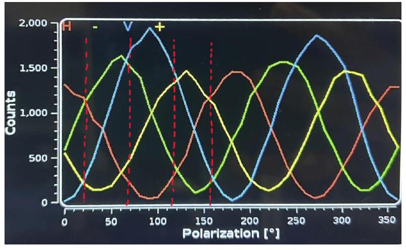
FIG. 15. Coincidence counts of the triplet state for one arm set at and the other swept in intervals of 10 degrees.
图15. 一个臂设置在,另一个以10度间隔扫描时三重态 的符合计数。
For the singlet state, on the other hand, we notice from figure 16 that i.) the coincidence counts are less (this agrees with our low visibility) and ii.) that the P and M curves are flipped compared to the singlet curves. As a result, i.) the magnitude of the expectation values in the basis (ie. and are smaller and ii.) they have an additional sign difference. This intuition agrees well with the experimental result we found in equation 64 where the and contributions are both negative and less than their theoretical maximum of . Therefore, both the quED apparatus and Bell's observable must be adjusted to improve coincidence rates and correct for sign changes respectively if we were to saturate Tsirelson's bound.
另一方面,对于单态,我们从图16注意到:i.) 的符合计数较少(这与我们的低可见度一致)和ii.) P和M曲线相对于单态曲线发生翻转。作为结果,i.) 基中期望值的幅度(即和较小,且ii.)它们具有额外的符号差异。这种直觉与我们在方程64中发现的实验结果很好地吻合,其中和的贡献都是负的,且小于它们的理论最大值。因此,如果我们要达到齐雷尔森界限,quED装置和贝尔可观测量都必须进行调整,分别用于改善符合率和校正符号变化。
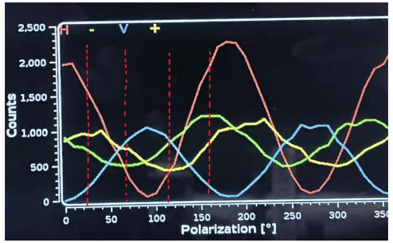
FIG. 16. Coincidence counts of the singlet state for one arm set at and the other swept in intervals of 10 degrees.
图16. 一个臂设置在,另一个以10度间隔扫描时单态 的符合计数。
VII. CONCLUSION VII. 结论
In this paper, we have explored the different polarizations of light and its transformations using Jones calculus. We have shown how maximally entangled photons can be produced using SPDC. We have reconstructed density and reduced density matrices using quantum state tomography and coincidence measurements. Above all, we have investigated the nature of light, experimentally tested Bell's inequality and verified that the full machinery of quantum mechanics is required to explain and understand photons. Just as how the theory of general relativity is necessary to describe systems in the presence of large masses, we have provided experimental evidence and hopefully a better understanding of how quantum mechanics is necessary to fully describe the complex behavior of light and entangled photons. Quantum mechanics is still very much a young and growing field. We have only begun to touch upon the tip of all there is to understand about this bizarre and unintuitive theory. There is still much to learn and uncover, but we hope that this paper establishes the experimental groundwork for all that there is to come.
在这篇论文中,我们探索了光的不同偏振及其使用琼斯演算的变换。我们展示了如何使用SPDC产生最大纠缠光子。我们使用量子态层析和符合测量重建了密度和约化密度矩阵。最重要的是,我们研究了光的本质,实验验证了贝尔不等式,并证实需要完整的量子力学机制来解释和理解光子。正如广义相对论理论对于描述存在大质量的系统是必要的一样,我们提供了实验证据,并希望能更好地理解为什么量子力学对于完整描述光和纠缠光子的复杂行为是必要的。量子力学仍然是一个非常年轻且正在发展的领域。我们才刚刚触及理解这个奇特且反直觉的理论的表面。还有很多需要学习和发现的地方,但我们希望这篇论文为未来所有的发展奠定了实验基础。
References
[1] A. G. Kofman. 在存在去相干和误差的情况下,贝尔不等式违反的最优条件。量子信息处理,11(1):269-309,2011年5月。
[2] Abraham G. Kofman 和 Alexander N. Korotkov. 超导相位量子比特中贝尔不等式违反的分析。物理评论B,77(10),2008年3月。